
Between artificial intelligence, data science, neural networks, and more, machine learning and its related fields have quickly become some of the biggest buzzwords in tech. With such a broad and exciting range of applications, machine learning has continued to grow into an all-solving black box, with a focus on what it can do instead of how it works. This article is the first in a series, in which we’ll explore the fundamentals of machine learning, and step through how a developer can implement these powerful tools for their projects. In the following posts, we’ll pivot to building models that specialize in time series prediction, and explore a variety of tools and techniques to improve our forecasting models.
If you’d like to follow along, the article is also available via Google Colab. Colab is an online hosted Jupyter Notebook that allows you to execute Python code right in your browser with no prior setup. Additionally, you can create, share, and edit Colab notebooks in Google Drive just as you would with any other Google Docs file.
A Primer in Machine Learning
In traditional programming, we typically input what we’ll call feature data, do a known computation on this data, and then return a result. We can represent that with this diagram.
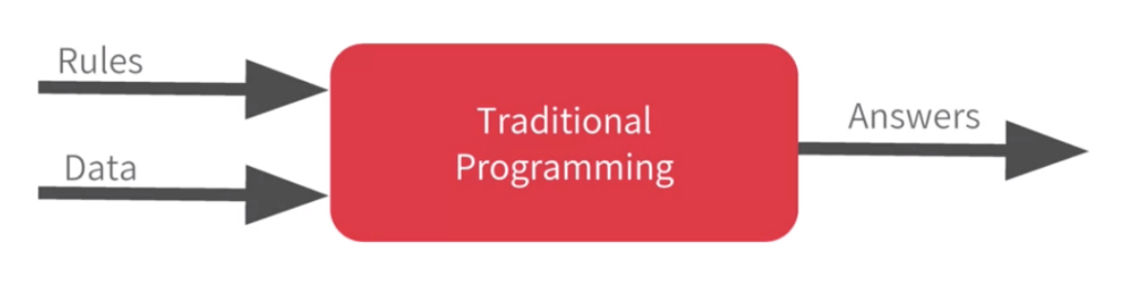
Here, the rules are expressed in whichever programming language we are using, and the output of our program is the answer.
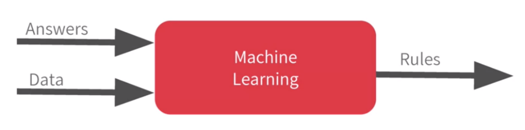
Machine learning rearranges this diagram. Here, we input labeled data, which includes both our known feature data and our answers, which we also call labels. We then get an approximation of the rules as our result.
Using a large batch of examples of what we want to see, machine learning models can get surprisingly accurate at approximating the rules that underlie our data. This is particularly useful for problems where we can’t fully define or understand the rules ourselves. For instance, how would I program the rules of what a cat looks like, or how would I write a program to translate every sentence of a book from one language into another? For such problems in the fields of computer vision, machine translation, and beyond, neural networks are an essential tool for generating solutions to complex problems. To begin, however, let’s look at a very simple example.
Our First Dataset: Laying the Groundwork for Time Series Prediction
Suppose we have a small data set of housing prices. This data includes only 2 variables, the size of the house in square meters, and the price of the house. We can say our feature data x representing the house’s size, and our label data y representing the price. For simplicity, we’ll represent both of these numbers in thousands:
x = [1, 1.5, 2.0, 2.5, 3.0]
y = [100, 140, 180, 220, 260]
After studying this data, you may have come to conclude that y = 80x + 20. To solve this, you might have noticed how when x increased by 1, y increased by 80. Then you might have seen that when x=1, y=100, and concluded that adding 20 solves the problem. Congratulations, you have quite the neural network in your head already! Machine learning works in a similar way, iterating over examples to understand the rules and patterns that govern them. If you wanted to define this rule yourself using traditional programming, you could simply write the following:
def price(size):
   return (80 * size) + 20

print(price(1.5))

> 140
Easy! But what if our dataset got a bit more descriptive? We might have size, the number of bedrooms, walkability score, and more, all factoring into the price by different amounts. Not only that, but some of these variables might be impacting one another, too! As these problems become more and more complex, the use of neural networks to learn the relationships becomes more attractive. For simplicity, however, let’s build a network to solve our basic example.
Building our First Neural Network with Time Series Prediction Capabilities
So far, we know that neural networks take in sets of labeled data, and iterate through it to train the network to accurately predict the solution. This training data is fed into the network in an input layer that is made up of neurons, where the number of neurons is equal to the dimensionality of the input data. You may have heard about how neural networks vaguely simulate the way the neurons in our brain work, but let’s take the “intelligent” out of this and focus on the “artificial”: a neuron is simply a node that holds a number.
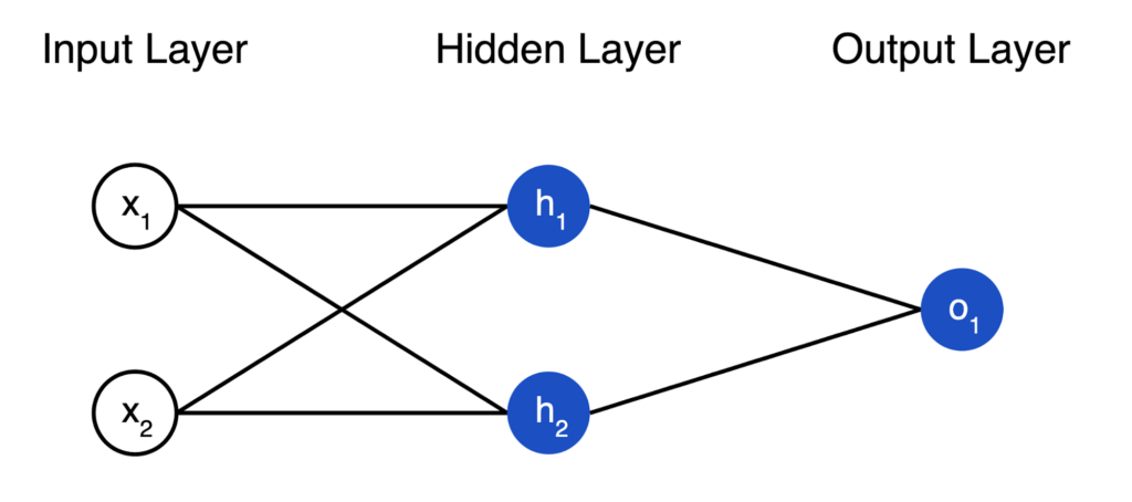
Next we have a hidden layer, which is another set of neurons that can be of any size you want. The neurons in the hidden layer are connected to the input layer via edges, each of which has a weight. To determine the value in any hidden neuron, we take the numbers in the input neurons, multiply them by their edge weights, and sum them up. We then take this sum and add a bias, which is a single value that is always applied to the neuron. Added together, if we define our edge weights as w and bias as b, the neuron’s final value could be defined as h = w(x) + b, with x being the values of the neurons in the previous layer. As we train our network, the weights on each edge will continuously adjust, in an attempt to more accurately approximate the answer.
Finally, we have the output layer, which is the response of our neural network. Just as the input layer has as many neurons as the dimensionality of our input data, the output layer has as many neurons as our output dimensionality. In our housing example, we’re inputting size and outputting price, so both our input and output layers will have just 1 neuron. In a classification example, for instance identifying pictures of digits 0 through 9, we would expect 10 neurons in the output layer.
Now that we have some idea of what we’re building, let’s get familiar with the different tools and libraries that will be used. The TensorFlow platform will provide all of the machine learning devices we will need. TensorFlow provides support for a few different programming languages such as C++, Java, and Python. For us, Python is a perfect fit with its immense volume of available libraries and straightforward syntax to start. Along with Python, we will be utilizing the NumPy library – NumPy gives us access to complex and fast data structures that will come in handy when feeding our data to our neural network. We’ll also use Keras, which is a framework in Tensorflow for defining neural networks. Let’s import those libraries now, and ensure that we’re running TensorFlow 2.5.
import tensorflow as tf
import numpy as np
from tensorflow import keras
print(tf.__version__)

> 2.5.0
Next we will create the simplest possible neural network using TensorFlow and Keras. It has 1 hidden layer with 1 neuron, and the input shape to it is just 1 value.
layer = tf.keras.layers.Dense(units=1, input_shape=[1])
model = tf.keras.Sequential([layer])
Next, we’ll need to give our network a loss function and an optimizer. Let’s get an idea of what those mean before storming ahead.
For any neural network, there is some defined function to measure how well the algorithm is performing. A loss function measures how well the algorithm performs on a single training example. The most basic loss function would simply get the difference between our predicted value ŷ, and the true value y.
Earlier, we concluded that y = 80x + 20. We could call our prediction function ŷ = w(x) + b, where we’re trying to solve for the best values of w and b. This equation may look familiar to you, it’s the same as how we calculate a neuron’s value! Just like our neuron’s equation, our home values are a combination of input values, weights on those inputs, and a bias. Our loss function could then be defined as J(w,b) = (y - ŷ)^2, the squared difference between our prediction and the true value. Our cost function is the average of our losses across a set of data, and we can call our cost function mean squared error (MSE). To visualize our equation, we could view J(w,b) as something like this:

The best values of w and b together minimize our loss, J(w,b), and are represented by the lowest point in the picture above. Suppose we started by guessing a random w and b in one of the far corners of the graph. How might we start moving towards the center?
Once a network checks how accurate its current prediction is, it must optimize its next prediction accordingly. It does so using an optimizer. In our housing example, we’re essentially trying to fit a line to our data, and one of the most common optimizers to do this is called stochastic gradient descent (SGD). We’ll spare you the math here, but we could visualize our optimizer as trying to move in the steepest downhill direction from our point (w,b), so as to minimize our loss for the next time series prediction. We’ll continue in a loop by making a prediction, measuring our loss, and optimizing for a specified number of steps, or epochs.
Now that we have an idea of what our loss function and optimizer are doing, let’s compile our neural network.
model.compile(optimizer='sgd', loss='mean_squared_error')
Training and Evaluating
Now, let’s again define our x and y arrays, this time as Numpy arrays. This is the standard data type we’ll want to use with our neural networks, as it can significantly improve performance. We’ll then train our neural network to this data using model.fit. Running this will make the network continuously loop through our data, making guesses, checking loss, and optimizing, for a specified number of epochs. We’ll have the model train for 500 epochs, and watch as the printed loss decreases rapidly.
x = np.array([1, 1.5, 2.0, 2.5, 3.0], dtype='float')
y = np.array([100, 140, 180, 220, 260], dtype='float')

model.fit(x, y, epochs=500)

>
Epoch 1/500
1/1 [==============================] - 1s 604ms/step - loss: 36037.2656
. . .
Epoch 500/500
1/1 [==============================] - 0s 10ms/step - loss: 3.3107
Since we independently defined our hidden layer earlier, we can actually look at the edge weights and biases that were applied to our hidden neuron! Using get_weights, let’s see what are values were after training.
print("Layer weights {}".format(layer.get_weights()))

> Layer weights [array([[77.66598]], dtype=float32), array([25.143635], dtype=float32)]
The first value here is weight applied to our input, while the second is the bias that’s added to the hidden neuron for every prediction. In other words, our network predicted our housing price equation to be about y = 77.7x + 25.1. It looks to have slightly undervalued the weight on x, while overvaluing the bias. Now that we’ve trained our network, we can use model.predict to see its prediction for any input value.
print(model.predict([1.5]))

> [[141.73691]]
Interesting – our weight and bias values were both off by a fair amount, but when predicting one of the values the network was trained on, it was quite accurate. Our model’s accuracy is hampered by how little data we fed it, but another issue we’ve fallen victim to is overfitting, in which our model is so fixated on the values it was trained on that it actually becomes less accurate in predicting new values.
How does our network do at predicting y for values of x that we didn’t include during training? To answer this question, we’ll introduce the idea of training and test sets. Commonly in machine learning, we want to withhold some of our data from training, and use it to evaluate the accuracy of our model. This withheld data is our test set, while everything we feed into the model is our training set. Let’s add a test set for our housing prices data, which will continue to increase the house size at the same interval. We can then test all of these values at once using model.predict.
x_test = np.array([3.5, 4.0, 4.5, 5.0], dtype='float')
y_test = np.array([300, 340, 380, 420], dtype='float')

print(model.predict(x_test))

> [[296.80087]
 [335.56686]
 [374.33286]
 [413.09885]]
As you might have known from our network’s weight and bias values, it becomes less and less accurate at predicting y as our x values increase, and move further away from what the network was trained on. As a final test, let’s modify our training and test sets, and see if it improves our network’s time series prediction across the full set of house sizes from 1 to 5. To do this, we’ll make a semi-random selection of what data goes into training and test, so it’s not all smaller values for training and larger for testing.
x = np.array([1.5, 2.0, 3.0, 3.5, 5.0], dtype='float')
y = np.array([140, 180, 260, 300, 420], dtype='float')

x_test = np.array([1.0, 2.5, 4.0, 4.5], dtype='float')
y_test = np.array([100, 220, 340, 380], dtype='float')

model.fit(x, y, epochs=500, verbose=0)

print("Layer weights {}".format(layer.get_weights()))

> Layer weights [array([[79.83571]], dtype=float32), array([20.567795], dtype=float32)]

print(model.predict(x_test))

> [[100.4035 ]
 [220.15706]
 [339.91064]
 [379.8285 ]]
Wow, our model’s weight and bias values are far more in line with the known values, and as such the time series prediction all improved drastically! This goes to show that beyond structuring a good network for the task at hand, we also need to think about how to organize our data to get optimal results.
In this article, we covered how neural networks can be trained with labeled data to learn and predict the underlying rules and relationships in the data. We saw how neurons calculate values, and propagate them through layers to produce an output, and how loss functions and optimizers are used to iteratively improve the network’s accuracy. We also saw how data is divided between training and test sets, and how properly splitting this data can improve network accuracy. In the next article in this series, we’ll apply all these concepts to a new data type, time series data, and explore how neural networks can be used to learn from history and forecast into the future.

About Mission Data
We’re designers, engineers, and strategists building innovative digital products that transform the way companies do business. Learn more: https://www.missiondata.com.